|
|

| ||
Demand
Much of the preceeding material in the consumer theory section is focused on the relationship between a consumer's preferences and a utility function that represents these preferences. There are two reasons for this emphasis. Preferences are a natural psychological concept. Faced with choice alternatives, it is reasonable to expect that a consumer will be able to rank the alternatives. But when economists evaluate markets, they would like to have a representation of demand. If preferences are represented by a utility function, then demand can be derived from maximization of utility for various prices and income. In this section, we assume that the consumer has preferences that are represented by a utility function, and we then carry out this derivation of demand. Once demand is represented by a function, it can be used to develop a model of exchange, and it can be combined with the supply functions of firms to model trade in a market.
Utility Functions
There are several classes of utility functions that are frequently used to generate demand functions. One of the most common is the Cobb-Douglas utility function, which has the form u(x, y) = x a y 1 - a. Another common form for utility is the Constant Elasticity of Substitution (CES) utility function. This function has the form u(x, y) = (a x r + b y r) 1/r. A third common utility function is quadratic, which has the form u(x, y) = 2 a x - (b - y) 2. Each of these utility functions has specific properties and uses which are discussed below after the demand function for each is derived.
Diminishing Marginal Rate of Substitution
Each of the utility functions examined below exhibits a property called "diminishing marginal rate of substitution." This means that as consumption of commodity X increases, the amount of another commodity that the consumer would give up to aquire an additional unit of X decreases. Figure 10 below demonstrates this idea. The curve in the figure shows a many combinations of commodities X and Y that all result in the same utility. Combinations of X and Y that produce the same utility level are called an "indifference curve." In figure 10, the combinations (x1, y1) = (3, 12), (x2, y2) = (4, 9), and (x3, y3) = (6, 6) all lead to the same level of utility. The marginal rate of substitution (MRS) going from (x1, y1) to (x2, y2) is 3, since the consumer is willing to give up 3 units of Y to get one additional unit of X. The MRS going from (x2, y2) to (x3, y3) is only 1.5, since the consumer is only willing to give up 3 units of Y to get 2 more units of X. This reduction in the marginal rate of substitution is one of the main assumptions about preferences or utility beyond the regularity assumptions that were described in earlier sections. Diminishing MRS is both an intuitive condition on preferences, and also a mild assumption, but in almost all cases it is enough to guarantee that the demand for a commodity decreases as its price increases.
Cobb - Douglas Utility
The Cobb-Douglas utility function has the form u(x, y) = x y for 0 < a < 1. Figure 10 shows combinations of commodities X and Y that result in the utility level u(x, y) = 6 for the Cobb-Douglas utility function u(x, y) = x y .
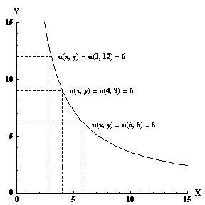
Figure 10: Indifference curve u(x, y) = 6 for the utility function u(x, y) = x 0.5 y 0.5.
For specific prices p x and p y and income M, the consumer has the budget equation p x x + p y y = M, where x and y are the levels of consumption of commodities X and Y. The optimal consumption level for each commodity is determined by setting the slope of the indifference curve through a point (x, y) equal to the slope of the budget line. Figure 11 shows two consumption points, 'a' and 'b'. At consumption point 'a', the slope of the indifference curve is not equal to the slope of the budget line. Note that at point 'b', the slope of the indifference curve and the budget line are equal, and the utility level is higher than at point 'a'.
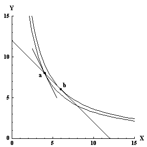
Figure 11: Non-optimal consumption point (a) and optimal point (b).
The top graph in figure 12 shows three example budget lines and the tangency, with the optimal consumption point for each. Since the price of X for each of the budget lines is different, and the optimal consumption level for X is different in each of the three cases, the relationship between px, the price of X, and the consumption level of X can be traced out. The lower graph in figure 12 traces out this relationship for a consumer with the indifference curves shown in the top portion of figure 12. In these graphs, the income is M = 120, the price of Y is fixed for all three budget lines at py = 10, and the price of X varies. The three prices for X are px = 12, px = 8, and px = 5. The optimal consumption level of commodity X when the price of X is px = 12 is indicated by the point labeled 'a' in the graph on the top portion of figure 12. Since the consumption level of X is x = 5 for px = 12, the price and quantity pair (x, p) = (5, 12) appears as the point labeled 'a' in the bottom graph in figure 12. The points labeled 'b' and 'c' in both graphs are interpreted similarly. The points 'a', 'b', and 'c' all lie on the demand graph, which is the bottom graph in figure 12.
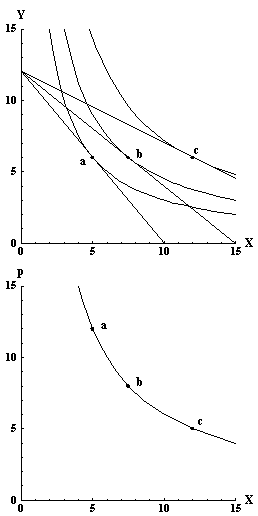
Figure 12: Optimal consumption points for three different prices (top) and corresponding demand function (bottom).
There is an important feature of the Cobb-Douglas utility function that is apparent in this figure. When the price of X changes, the demand for Y doesn't change. This means that commodities X and Y are neither substitutes for one another nor complements to one another.
| Derived demand for Cobb-Douglas utility |
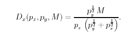
| The graphical derivation of demand described above is useful for understanding what it means to derive demand from a consumer's utility and budget, but an analytical technique is helpful since the demand is then known for many different income levels and for different prices of the other commmodity Y. The analysis below shows how this is done for the Cobb-Douglas utility function. The simplest way to find the slope of the indifference curve is to use implicit differentiation. In implicit differentiation, y is written as y(x) so that on the indifference curve with utility level c, x y(x) = c. When this is differentiated with respect to x, the result is The budget line can be rewritten as y = M / py - (px / py) x, so its slope is -px / py. When the slope of the indifference curve, which is a y / (1 - a) x, is set equal to the slope of the budget equation, the result is (1 - a) p y y = a p x x. This tangency condition can be substituted into the budget equation to eliminate either x or y so that the demand for one of the commodities can be obtained. Substitute p x x = ((1 - a)/a) p y y into p x x + p y y = M to get (1 + (1 - a)/a) p y y = M. Then the demand for Y is y(p y, M) = a M/p y. |
CES Utility
The Constant Elasticity of Substitution (CES) utility function is useful because this class of utility functions can be used to model commodities that are either substitutes for one another, or complements of one another. The CES utility function for two commodities X and Y can be written u(x, y) = (a x r + b y r) 1/r for any values of a > 0, b >0, and r < 1 and r  0.
0.
Derived demand for CES utility
The technique for determining demand functions is similar to the technique that was used above to determine the demand for the Cobb-Douglas utility function. The first step is to determine the slope of the indifference curve through a given point (x, y), and then set the slope of the indifference curve through (x, y) equal to the slope of the budget equation.
The most elementary technique for finding the slope of the indifference curve through (x, y) is to differentiate the equation u(x, y) = c implicitly. The slope of the indifference curve is 1/r (a x r + b y r) 1/r - 1 (r a x r - 1 + r b y r - 1 dy/dx) = 0. For (x, y) (0, 0), this expresion holds if and only if dy/dx = -(a x r - 1)/(b y r - 1). The slope of the budget line is -p x/p y, so the tangency condition is b p x x 1 - r = a p y y 1 - r or
Once the last equation is solved for p y y and the result is substituted into the budget equation, the demand for commodity X is easily obtained by solving for x. This demand function is
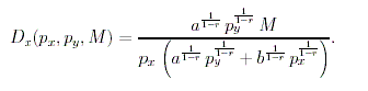
Example CES utility and demand functions
If the parameters in the CES utility function are a = 1, b = 1, and r = -1, then the utility function is u(x, y) = (x -1 + y -1) -1 and the demand function can be obtained by substituting a = 1, b = 1, and r = -1 into the demand equation above. This results in
Quadratic Utility
u(x, y) = 2 a x - (b - y) 2
| Copyright 2006 Experimental Economics Center. All rights reserved. | Send us feedback |