(In the lecture material below, supply and demand are developed jointly. Some teachers, however, will prefer to do demand in its entirety and then supply and thus we separate out the sections to allow a teacher to rearrange the text below to allow for separate presentations.)

1. Definitions
2. Demand Curve
3. Supply Curve
4. Transition into Competitive Equilibrium Theory
5. Extensions

Begin with some basic definitions and the sorted tables generated by the experiment.

Definition: The market for any good or service consists of all (actual or potential) buyers or sellers of that good or service.

In the first M&M experiment, the market consisted of 1 seller (me) and ## buyers (you). In the second experiment, the market consisted of 1 buyer (me) and ## sellers (you).

Demand:

Start with discussing the demand table generated by the first experiment and what it means.

In the first M&M experiment, buyers had to decide their reservation prices: the maximum amount of money that would be willing to pay to obtain a packet of M&Ms (the highest price at which he or she would be willing to buy my packet rather than not buy it). If you bought a packet, you would incur a cost equal to the price called out in the auction and receive whatever your reservation price was as a benefit: the market price represented the marginal cost and your reservation price was the marginal benefit. The difference between these two values is the economic surplus you would gain from purchasing a packet.

The teacher can now use the table to demonstrate for any price how many units of M&Ms would be purchased (demanded) and determine for any quantity the price that would lead to that quantity being purchased (demanded).

The teacher can tie this back to what was actually observed in the auction: To sell three packets, what price would have to be set? What price did the three packets sell for? Point out a price at which fewer than 3 students were willing to purchase a packet (excess supply). Point out a price at which more than 3 students were willing to purchase a packet (excess demand).

Supply:

Now discuss the supply table generated by the second experiment and what it means.

In the second M&M experiment, sellers had to decide their reservation prices: the minimum amount of money that would compensate them for giving up the packet of M&Ms (the lowest price at which he or she would be willing to sell your packet rather than not sell it at all). If you sold a packet, you would receive the price called out in the auction and incur whatever your reservation price was as a cost: the market price represented the marginal benefit and your reservation price was the marginal cost. The difference between these two values is the economic surplus you would gain from selling a packet.

The teacher can now use the table to demonstrate for any price how many units of M&Ms would be sold (supplied) and determine for any quantity the price that would lead to that quantity being sold (supplied).

The teacher can tie this back to what was actually observed in the auction: To buy three packets, what price would have to be set? What price did the three packets sell for? Point out a price at which fewer than 3 students were willing to sell a packet (excess demand). Point out a price at which more than 3 students were willing to sell a packet (excess supply).

Return to the sorted demand table.

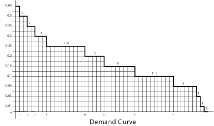
Note that we can visually present the values from this table in what economists call a demand curve. Below is an example of a demand curve generated from a class of 50 students. In this auction, three units were sold at 50 cents per unit.

Definition: The demand curve for a good or service tells us the total quantity of that good or service that buyers wish to buy at each price.

The demand curve is the set of all price-quantity pairs for which buyers are satisfied. ("Satisfied" means being able to buy the amount they want to at any given price.)

We can draw a demand curve when we know each buyer's reservation price.

Explain how to read the step curve. By convention, we put price on the vertical axis and quantity on the horizontal axis. Like in the table, we order the information from high-value buyers to low-value buyers. $0.65 is the most any buyer would pay for a packet (so for all prices above $0.65, the number of units demanded is 0). One buyer is willing to pay up to $0.65 to buy one packet. Point out a few prices and ask them how many units would be demanded in the classroom market at this price. Point out a few quantities and ask at what price would buyers be willing to buy this many units. Note how the answers are the same as in when we discussed the table. Remind them of the price at which 3 packets were purchased and point this price-quantity pair out on the graph.

Some teachers may wish to introduce (or re-introduce) the concept of economic surplus and show how it is represented by an area.

Note that a demand curve is just a visualization of marginal benefits. Point out how each segment on the graph corresponds to the "marginal benefit" to the economy of purchasing one more unit.

Notice that our classroom demand curve is a step curve. In your book and in later lectures, the demand curves are presented as straight lines. In reality, most demand curves are steps, but straight lines are a very good approximation. With many buyers and many sellers trading thousands or millions of units, or units that are perfectly divisible, the steps would be so tiny as to be not worth drawing. The straight line is much easier to draw and manipulate (similar to Production Possibility Curves, which are typically faceted surfaces but we often use smooth curved lines to represent them).

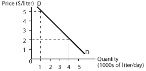
On the board (or in a handout) draw the demand curve for milk:

If the price were $2/liter, buyers would demand 4000 liters per day. Another way of looking at it: the demand curve tells us that the marginal benefit from consuming the 4000th liter of milk is $2 If milk suppliers only desired to sell 1000 liters of milk per day, they could charge as high as $5/liter.



Underlying concept: People should be willing to buy a good or service as long as the price is less than or equal to the benefit they derive.

Demand curves slope downward for three reasons:

1. As the good becomes more expensive, people switch to substitutes.
2. As the good becomes more expensive, people can't afford to buy as much of it.
3. As an individual consumes more of a good, at some point his or her marginal benefit from consuming an additional unit will decline (can conduct a thought experiment at this point in lecture: what might the demand curve have looked like if we had we run the supply experiment immediately before the demand experiment - i.e., if we had given each student a free packet of M&Ms and asked for the maximum price at which they would be willing to purchase another packet?).

Return to the sorted supply table.

Note that we can visually present the values from this table in what economists call a supply curve.

Definition: The supply curve of a good or service tells us the total quantity of that good or service that sellers wish to sell at each price.

The supply curve is the set of price-quantity pairs for which sellers are satisfied. ("Satisfied" means being able to sell the amount they want to at any given price.)

We can draw a supply curve when we know each buyer's reservation price.

Explain how to read the supply curve. Point out a few prices and ask them how many units would be supplied in the classroom market at this price. Point out a few quantities and ask at what price would sellers be willing to sell this many units. Note how the answers are the same as in when we discussed the table. Remind them of the price at which 3 packets were purchased and point this price-quantity pair out on the graph.

Some teachers may wish to introduce (or re-introduce) the concept of economic surplus and show how it is represented by an area.

Note that a supply curve is just a visualization of marginal costs. Point out how each segment on the graph corresponds to the "marginal costs" to the economy of selling one more unit.

Notice that our classroom supply curve, like our classroom demand curve, is a step curve. In your book and in later lectures, the supply curves are presented as straight lines for the same reasons we will present demand curves as straight lines: because straight lines are easier to draw and are a very good approximation of the step curves.

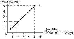
On the board (or in a handout) draw the supply curve for milk:

If the price were $2/liter, sellers would be willing to supply 2000 liters per day. Another way of looking at it: the supply curve tells us that the marginal cost of producing the 2000th liter of milk is $2. In other words, the opportunity cost of producing this last liter is $2. If market price was $5 per liter, suppliers would want to supply 5000 liters.

Underlying concept: People should be willing to sell milk as long as the price they receive is sufficient to cover the opportunity costs of supplying it. So if what they could earn by selling milk is not sufficient to compensate them for what they could have earned had they spent their time and resources elsewhere, they won't sell milk.

Why does the supply curve slope upward? Two general reasons: (1) as we expand the production of any good, we turn first to those people and resources whose opportunity costs of producing that good are lowest, and only then to others with higher opportunity costs. The higher the price for milk, the more likely that resources that are relatively less efficient at producing milk will be employed to produce milk; (2) The marginal cost of producing a good often rises as we produce more of it.

In the case of our market for M&Ms, the opportunity cost of supplying a packet of M&M was the perceived foregone benefit from not having the packet. If the market price were higher than this perceived benefit, an individual would give up the packet in exchange for the cash. Thus the supply curve slopes upwards because some people have higher perceived benefits from retaining the M&M packet than others.

Pose the following question to students, "How might 'classroom trade' have been conducted if an auction were not used (e.g., command and control; unorganized bilateral bargaining; posted offers; double auction)?" This discussion then leads naturally into competitive equilibrium theory and double auction experiments.

Economists model information on marginal benefits and marginal costs as supply and demand curves, which help us predict how many units are likely to be sold and at what price.

What might happen in the supply experiment if instead of me purchasing the packets through an auction, we brought in another classroom of students with the same marginal benefits for packets of M&Ms as your class (in other words, the same demand curve) and allowed the two classes to trade?

Project the M&M supply and demand experimental curves on the same graph.

Would three have been sold? More? Less? We would expect trade to take place as long as buyers could buy packets at prices less than or equal to their reservation prices (marginal benefits) and sellers could sell packets at prices greater than or equal to their reservation prices (marginal costs).

There is no reason to believe that at any arbitrary price (say $0.55), the number of packets that buyers want will be equal to the number of packets that sellers would be willing to sell at that price. But there is a price at which this is true. This price, at which "supply equals demand," is called the competitive equilibrium price and the number of units bought and sold at this price is called the competitive equilibrium quantity. Equilibrium occurs at the price-quantity pair for which both buyers and sellers are satisfied.

A market is in equilibrium when no participant in the market has an incentive to alter his or her behavior and thus there is no tendency for production or prices to change in that market.

Can return to the demand and supply curves to talk about:

1. movements along the demand curve (changing how many were purchased or sold in auctions) versus changes in demand and supply;
2. to talk about taxes and subsidies (what would have happened if I charged a 10 cent tax to anyone who sold a packet of M&Ms in the reverse English auction?);
3. to talk about monopoly (what if someone controlled the entire supply of M&Ms but the demand curve comprised competitive buyers?);
4. to talk about price ceilings and price floors.